In this post, we will implement an algorithm for the K-Means problem and visualize it with a Matplotlib animation.
A mathematical introduction
In the K-Means problem, a set of $n$ observations $X = {x_1, \ldots, x_n}$, with $x_i \in \mathbb R^d$, is given. The goal is to partition the set $X$ into $k$ sets $S = {S_1, \ldots, S_k}$, such that the total energy is minimized. We define the energy of the $i$-th cluster as follows:
$$E(i) = \sum_{x_j \in S_i} {|x_j - \mu_i|}^2,$$
where $\mu_i$ is a chosen representative of the cluster $S_i$. Usually $\mu_i$ is taken to be the centroid of cluster $i$, that is, the mean of all the points in $S_i$. In symbols, the objective is to find
$$\mathop{\mathrm{arg,min}}\limits_{S} \sum_{i = 1}^k E(i).$$
This problem is computationally difficult (NP-hard): even though most algorithms do reasonably well, they usually converge to a local minimum. For such a solution, every minor rearrangement of the clusters makes the energy grow. However, there could be a completely different clustering where the total energy would be even lower. For this reason, those algorithms are called ‘heuristic’.
Lloyd’s algorithm
We will implement one of the simplest algorithms for the K-Means problem, known as the Lloyd’s algorithm. It is an iterative algorithm that, given an initial estimate of the centroids $\mu_i$, progresses by repeating two steps:
- Assignment: each point is assigned to the cluster whose centroid gives the smallest energy. Since we are working in $\mathbb R^d$, it’s worth noting that if we assume the norm $|\cdot|$ to be the standard Euclidean norm, then the energy of a cluster is nothing else but the sum of the distances between each point in the cluster and the centroid. In this case it’s possible to think of this step as the assignment of each point to the nearest centroid.
- Update: for each cluster, a new centroid is calculated:
$$\mu_i = \mathop{\mathrm{arg,min}}\limits_{\hat\mu} \sum_{x_j \in S_i} {|x_j - \hat\mu|}^2$$
Observe that in the second step the function to minimize is differentiable: in other words, $\mu_i$ satisfies
$$2\sum_{x_j \in S_i} |x_j - \mu_i| = 0.$$
Since the mean of the points in $S_i$ satisfies that condition, we can simply choose
$$\mu_i = \frac1{|S_i|} \sum_{x_j \in S_i} x_j.$$
Finally, it’s interesting to observe that the above algorithm does indeed converge to a local minimum. The first step decreases the total energy by construction, and so does the second one because the mean is a least-squares estimator, as we have seen. Moreover, the energy is nonnegative. It follows that the energy function has a minimum. But we can prove more: given a set of centroids ${\mu_i}$, the assignment step yields either the same clustering or a clustering with lower energy. Since there are at most $k^n$ ways to partition the $n$ observations into $k$ clusters, a local minimum will be reached in a finite number of iterations.
Algorithm implementation
The Lloyd’s algorithm requires initial estimates for the centroids. There are several ways to provide such values. We will simply take $k$ samples from the data. Let’s define a function for that:
import numpy as np

def random_sample(X, k):
    return X[np.random.choice(X.shape[0], k, replace=False),:]
Now we need a function to compute the distance between each point and all the centroids. We will keep track of the index of the centroid that yields the lowest distance.
def pairwise_distances_argmin(X, y):
    indices = np.empty(X.shape[0], dtype=np.intp)
    for i in range(len(X)):
        indices[i] = np.linalg.norm(X[i,np.newaxis] - y, axis=1).argmin()
    return indices
As an example, consider the points $X = {(0, 0), (5, 5)}$ and the centroids $\mu = {(1, 1), (6, 6)}$. The first point is then closer to the first centroid, while the second point is closer to the second centroid:
X = np.array([[0, 0], [5, 5]])
y = np.array([[1, 1], [6, 6]])
pairwise_distances_argmin(X, y)
array([0, 1])
The result is an array of indices, and we can effectively interpret it as a set of cluster labels: the first point belongs to cluster “$0$”, the second point to cluster “$1$”. This is the first step of Lloyd’s algorithm. We can now implement the second step and wrap them together in a single function, which will execute a complete iteration of Lloyd’s algorithm.
def kmeans_iteration(X, m):
    clusters = pairwise_distances_argmin(X, m)
    centroids = np.empty(m.shape)
    for i in range(len(m)):
        centroids[i] = np.mean(X[clusters == i], axis=0)
    return centroids, clusters
For each cluster, we simply compute the mean of the points belonging to that cluster. The results are the new clusters. To complete the implementation, we need to iterate the above until convergence is achieved and a local solution is found.
def kmeans(X, k):
    m = random_sample(X, k)
    while True:
        new_m, clusters = kmeans_iteration(X, m)
        if np.isclose(m, new_m).all():
            break
        m = new_m
    return new_m, clusters
In the minimal implementation above, we chose to check whether the updated centroids are very close to each other: the np.isclose function compares value with default tolerances of $10^{-5}$ and $10^{-8}$. Those are, respectively, the relative tolerance and the absolute tolerance. We want to avoid strict equality because floating point math is not exact. I encourage you to read Goldberg’s “What Every Computer Scientist Should Know About Floating-Point Arithmetic” if you want to examine this topic in greater depth.
There are other ways in which we could have interrupted the algorithm: we can impose a maximum number of iterations, or stop once the total energy of the clusters has gone below a certain threshold.
Now let’s visualize the result of the algorithm.
import matplotlib.pyplot as plt
import matplotlib.cm as cm
from matplotlib import rc
import seaborn as sns

plt.style.use('ggplot')
sns.set_style('whitegrid')
rc('figure', figsize=(6, 4))
cmap = cm.get_cmap('rainbow')

def plot_clusters(X, m, clusters):
    k = len(m)
    for i in range(k):
        group = X[clusters == i]
        plt.scatter(group[:,0], group[:,1], marker='.', color=cmap(i / k))
        plt.scatter(m[i,0], m[i,1], marker='*', color=cmap(i / k))
    plt.show()
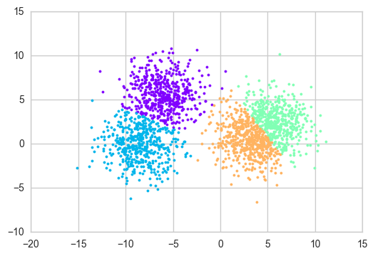
We’ll generate the data with the function make_blobs from scikit-learn.
from sklearn.datasets import make_blobs

X, _ = make_blobs(n_samples=2000, centers=4, cluster_std=2)
m, clusters = kmeans(X, 4)
plot_clusters(X, m, clusters)
Now let’s generate an animation showing the steps of Lloyd’s algorithm. We’ll use the FuncAnimation class from Matplotlib. It requires a function to update the data repeatedly. Since each iteration of the algorithm depends upon the previous iteration, we’ll create a class to keep track of the state.
import matplotlib.animation as animation

class KMeansAnimation:
    def __init__(self, fig, ax, X, m=None, k=2):
        self.X = X
        self.fig = fig
        self.m = m if m is not None else random_sample(X, k)
        # We have to call plot for each cluster and its centroid
        # because we want to distinguish the clusters by color
        # and draw the centroid with a different marker
        self.clusters, self.centroids = [], []
        for i in range(k):
            color = cmap(i / k)
            self.clusters.append(
                ax.plot([], [],
                        linestyle='', marker='.',
                        markeredgecolor=color, color=color)[0]
            )
            self.centroids.append(
                ax.plot([], [],
                        linestyle='', marker='o',
                        markeredgewidth=0.5,
                        markersize=10, color=color)[0]
            )

    def update(self, t):
        self.m, clusters = kmeans_iteration(self.X, self.m)
        self.fig.suptitle('n = {}, k = {} – Iteration {}'.format(
                len(self.X), len(self.m), t + 1)
        )
        # To update the plot, we simply call set_data on the saved axes
        for i in range(len(self.m)):
            group = self.X[clusters == i]
            self.clusters[i].set_data(group.T)
            self.centroids[i].set_data(self.m[i])
        return self.clusters + self.centroids
We create a convenience function that generate HTML code to embed the animation as a <video> element.
from IPython.display import HTML

def make_animation(X, k, m=None, frames=20):
    fig = plt.figure(figsize=(6, 4))
    (xmin, ymin), (xmax, ymax) = np.min(X, axis=0), np.max(X, axis=0)
    ax = plt.axes(xlim=(xmin, xmax), ylim=(ymin, ymax))
    control = KMeansAnimation(fig, ax, X, m=m, k=k)
    anim = animation.FuncAnimation(
        fig, control.update,
        frames=frames, interval=700, blit=True,
    )
    # Necessary, otherwise the notebook will display the final figure
    # along with the animation
    plt.close(fig)
    return HTML(anim.to_html5_video())
For this we will generate some more blobs and use less clusters than the number of blobs to better see the algorithm in action.
from sklearn.datasets import make_blobs

X, _ = make_blobs(n_samples=2000, centers=6, cluster_std=2.2)
Let’s check the blobs first. They are not immediately recognizable due to the high variance we introduced.
plt.plot(X[:,0], X[:,1],
         linestyle='', marker='.',
         color=cmap(0.2), markeredgecolor=cmap(0.25))
plt.show()
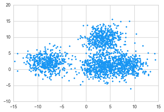
We’ll manually choose the starting centroids, and we will choose them in such a way that at least two of them are very close. This will make for a tougher problem for Lloyd’s algorithm. This will represent an uncommon situation: usually choosing the initial centroids at random will give it much better chances to perform well.
m = np.array([[0, 2.5], [3, 11], [4, 10], [5.5, 2]])
make_animation(X, m=m, k=4, frames=20)
It’s fascinating to observe the journey of the green (or ‘seafoam green’, according to XKCD) centroid: since the algorithm tends to put some distance between the centroids, if two centroids start too close one of them will be eventually moved farther away.
Let’s see what happens when we run the algorithm on a uniformly populated area:
X_dense = np.random.rand(2000, 2)
make_animation(X_dense, k=11)
As we can see, Lloyd’s algorithm tends to partition the space into clusters of uniform area. After running the algorithm on a dense space, it should be clear that Lloyd’s algorithm is closely related to Voronoi diagrams. In fact, at each iteration we are effectively computing the Voronoi tessellation with respect to the centroids.
Bonus: how to choose $k$?
We never mentioned how one should choose the parameter $k$. After all, this algorithm is used for unsupervised learning, and the number of cluster is not necessarily known a priori. This is actually a non-trivial problem and there are a number of ways to approach it. A relatively recent result is represented by the Gap statistics (PDF), a method developed by Tibshirani, Walther and Hastie in 2001.
Let $W_k$ be the total energy of the clusters, when $X$ is partitioned into $k$ clusters:
$$W_k = \sum_{i = 1}^k E(i) = \sum_{i = 1}^k \sum_{x_j \in S_i} {|x_j - \mu_i|}^2.$$
The idea behind their method is make a standardized comparison between $\log W_k$ and a null reference distribution of the data; that is, a distribution with no clear clustering. The authors claim that the optimal number of clusters is the value of $k$ for which $\log W_k$ falls the farthest below the reference curve. This information is embedded in what they call “gap statistic”:
$$\mathop{\mathrm{Gap}}_n(k) = E_n^*{\log W_k^*} - \log W_k.$$
Here $E_n^*$ denotes the expected value under a sample of size $n$ from the reference distribution. The estimate $\hat k$ will then be the value of $k$ that maximizes $\mathop{\mathrm{Gap}}_n(k)$, after having taken the sample distribution into account.
Algorithm implementation
To generate the reference distribution, the paper suggests two alternatives:
a) Monte Carlo sampling over the bounding box of the data; b) random sampling over a box aligned with the principal components of the data.
Even though route b) is more robust, it requires a singular value decomposition of the matrix $X$. We are going to choose the first option for its simplicity of implementation.
The implementation follows these steps:
- cluster the data with $k = 1, \ldots, K$, and computing for each partition the total energy $W_k$;
- generate $B$ reference data sets, computing for each one the total energy $W_{bk}^*$.
Then the gap will be
$$\mathop{\mathrm{Gap}}(k) = \frac1B\sum_{b = 1}^B \log W_{bk}^* - \log W_k,$$
where the first term is the mean of the log-energies $\log W_{bk}^*$ of the samples. We also have to account for the simulation error: if $\mathop{\mathrm{sd}}(k)$ denotes the standard deviation of the log-energies $\log W_k^*$, then the error is
$$s_k = \mathop{\mathrm{sd}}(k)\sqrt{1 + \frac1B}.$$
Finally, the optimal cluster size $\hat k$ is the smallest $k$ such that $\mathop{\mathrm{Gap}}(k) \geq \mathop{\mathrm{Gap}}(k + 1) - s_{k + 1}$, or $\mathop{\mathrm{Gap}}(k) - \mathop{\mathrm{Gap}}(k + 1) + s_{k + 1} \geq 0.$
Let’s start by implementing a function to calculate the total energy of a clustering:
def Wk(X, centroids, clusters):
    return np.sum([np.linalg.norm(X[i] - centroids[clusters[i]]) ** 2
                   for i in range(len(X))])
We’ll also need a function to take uniform samples from the observations $X$:
def monte_carlo(X, xmin, xmax, ymin, ymax, n=None):
    # n is the sample size
    n = n if n is not None else len(X)
    xs = np.random.uniform(xmin, xmax, size=(n, 1))
    ys = np.random.uniform(ymin, ymax, size=(n, 1))
    return np.concatenate([xs, ys], axis=1)
Now we can implement the rest of the algorithm.
def gap_stats(X, K=8, B=10, n=None):
    (xmin, ymin), (xmax, ymax) = np.min(X, axis=0), np.max(X, axis=0)
    ks = np.arange(1, K + 1)
    # Generate B Monte Carlo samples (uniform) from the bounding box of X
    samples = [monte_carlo(X, xmin, xmax, ymin, ymax, n) for _ in range(B)]
    # Total energy of X for each k
    Wks = np.empty(K)
    # Mean total energy of samples for each k
    sample_Wks = np.empty(K)
    # Corrected standard deviation for each k
    sk = np.empty(K)
    for k in ks:
        Wks[k - 1] = np.log(Wk(X, *kmeans(X, k)))
        # Total energy for each sample
        current_Wks = np.empty(B)
        for i in range(B):
            sample = samples[i]
            current_Wks[i] = np.log(Wk(sample, *kmeans(sample, k)))
        sample_Wks[k - 1] = current_Wks.mean()
        sk[k - 1] = np.sqrt(((current_Wks - sample_Wks[k - 1]) ** 2).mean())
    # Correction factor
    sk *= np.sqrt(1 + 1 / B)
    gaps = sample_Wks - Wks
    return ks, Wks, sample_Wks, gaps, sk
We want to test the above algorithm on different configurations of points. We’ll first make a function to summarize the gap statistics for a certain distribution.
import matplotlib.ticker as ticker

def gaps_info(X, ks, Wks, sample_Wks, gaps, sk):
    fig, axes = plt.subplots(2, 2, figsize=(8, 7))
    axes[0,0].plot(X[:,0], X[:,1],
                   linestyle='', marker='.',
                   color=cmap(0.2), markeredgecolor=cmap(0.25))
    line1, = axes[0,1].plot(ks, Wks, marker='.', markersize=10)
    line2, = axes[0,1].plot(ks, sample_Wks, marker='.', markersize=10)
    axes[0,1].legend(
        (line1, line2),
        (r'$\log W_k$', r'$\frac{1}{B}\sum_{b = 1}^B\,\log W_{kb}^*$')
    )
    axes[1,0].plot(ks, gaps, marker='.', markersize=10)
    axes[1,0].set_ylabel('$\mathop{\mathrm{Gap}}(k)$')
    gaps_diff = gaps[:-1] - gaps[1:] + sk[1:]
    barlist = axes[1,1].bar(ks[:-1], gaps_diff,
                            width=0.5, align='center')
    barlist[np.argmax(gaps_diff > 0)].set_color(sns.xkcd_rgb['pale red'])
    axes[1,1].set_ylabel('$\mathop{\mathrm{Gap}}(k) -'
                         ' \mathop{\mathrm{Gap}}(k + 1) + s_{k + 1}$')
    for (i, j) in ((0, 1), (1, 0), (1, 1)):
        axes[i,j].set_xlabel('Clusters')
        axes[i,j].xaxis.set_major_locator(ticker.MaxNLocator(integer=True))
    fig.tight_layout(w_pad=3)
    plt.show()
Let’s start with an easy one. We’ll use the make_blobs function from before to make three very distinguishable clusters.
X, _ = make_blobs(n_samples=1000, centers=3, cluster_std=2)
ks, Wks, sample_Wks, gaps, sk = gap_stats(X, K=5)
gaps_info(X, ks, Wks, sample_Wks, gaps, sk)
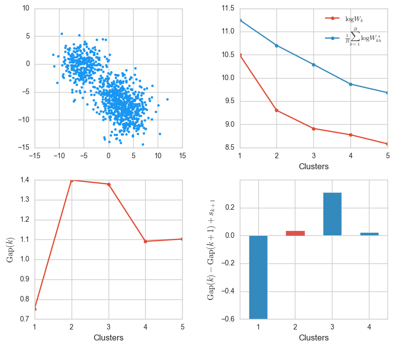
The value $k = 2$ corresponds to the maximum $\mathop{\mathrm{Gap}}$, and we see that it’s also the lowest value for which $\mathop{\mathrm{Gap}}(k) - \mathop{\mathrm{Gap}}(k + 1) + s_{k + 1}$ is positive. This confirms that $k = 2$ is indeed optimal.
Let’s see what happens when we increase the standard deviation when generating blobs.
X, _ = make_blobs(n_samples=1000, centers=3, cluster_std=2.8)
ks, Wks, sample_Wks, gaps, sk = gap_stats(X, K=5)
gaps_info(X, ks, Wks, sample_Wks, gaps, sk)
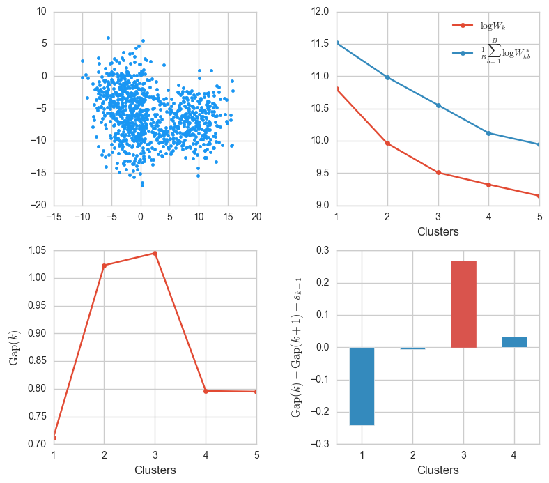
The clusters are close and slightly fused, that even though they were generated from three centers, they could look like two clusters. The algorithm, though, correctly determines that $k = 3$ is the best value.
Until now we have only tried the algorithm up to $k = 5$ candidate clusters. Let’s see how the algorithm responds to a configuration with more blobs and more candidates.
X, _ = make_blobs(n_samples=1000, centers=8)
ks, Wks, sample_Wks, gaps, sk = gap_stats(X, K=12)
gaps_info(X, ks, Wks, sample_Wks, gaps, sk)
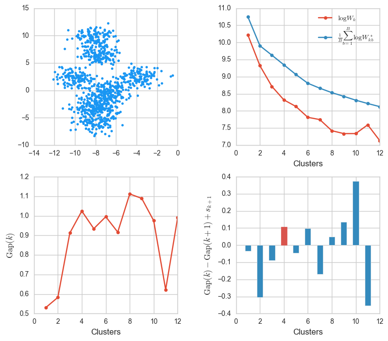
This was tricky. The blobs were generated from eight centers but some of them fused and in the end only four or five are visible. The algorithm determined that $k = 4$ was best.
On the other hand, it’s also very interesting to test the algorithm with one single cluster.
X, _ = make_blobs(n_samples=600, centers=1, cluster_std=4)
ks, Wks, sample_Wks, gaps, sk = gap_stats(X, K=5)
gaps_info(X, ks, Wks, sample_Wks, gaps, sk)
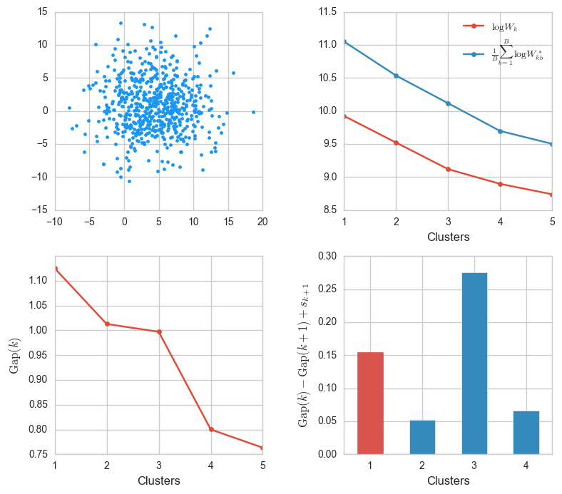
The algorithm concludes without problems that $k = 1$ is best. Note that in the top rightmost plot, the energy of the observed data falls at roughly the same rate as the energy from the uniform samples. That makes sense, since a Gaussian distribution (the one from which the blobs are generated) can be approximated by the uniform distribution on an interval, progressively better as the standard deviation increases.
As the last example, let’s consider a uniform sample, to see what the algorithm decides.
X = np.random.uniform(-10, 10, size=(600, 2))
ks, Wks, sample_Wks, gaps, sk = gap_stats(X, K=4)
gaps_info(X, ks, Wks, sample_Wks, gaps, sk)
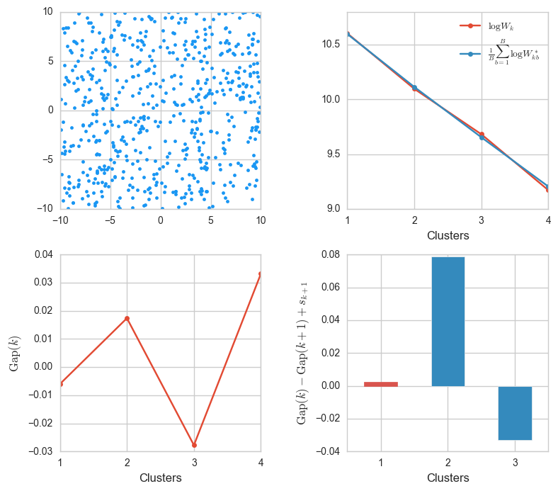
This confirms what we anticipated in the last example: now the energy decay is almost identical. That’s because the distribution of the observed data and the samples is exactly the same.
Conclusion
In this notebook we introduced the K-Means problem and implemented Lloyd’s algorithm, one out of the several that exist to solve it. We then animated the steps of Lloyd’s algorithm with Matplotlib. Finally, we tackled the problem of determining the optimal number of clusters, and implemented the ‘gap statistics’ from the Tibshirani, Walther and Hastie paper. This algorithm proved to be quite reliable, having successfully determined the optimal number of clusters in all of the different cases we tested it on.
