
A BK-tree is a tree data structure specialized to index data in a metric space. A metric space is essentially a set of objects which we equip with a distance function $d(a, b)$ for every pair of elements $(a, b)$. This distance function must satisfy a set of axioms in order to ensure it’s well-behaved. The exact reason why this is required will be explained in the “Search” paragraph below.
The BK-tree data structure was proposed by Burkhard and Keller in 1973 as a solution to the problem of searching a set of keys to find a key which is closest to a given query key. The naive way to solve this problem is to simply compare the query key with every element of the set; if the comparison is done in constant time, this solution is $O(n)$. On the other hand, a BK-tree is likely to allow fewer comparisons to be made.
Construction of the tree
BK-tree is defined in the following way. An arbitrary element $a$ is selected as root. Root may have zero or more sub-trees. The $k$-th sub-tree is recursively built of all elements $b$ such that $d(a,b) = k$.
To see how to construct a BK-tree, let’s use a real scenario. We have a dictionary of words and we want to find those that are most similar to a given query word. To gauge how similar two words are, we are going to use the Levenshtein distance. Essentially, it’s the minimum number of single-character edits (which can be insertions, deletions or substitutions) required to mutate one word into the other. For example, the distance between “soccer” and “otter” is $3$, because we can change the first one into the other by deleting the leading s, and then substituting the two central c’s with two t’s.
Let’s use the dictionary
{'some', 'soft', 'same', 'mole', 'soda', 'salmon'}
To construct the tree, we first choose any word as the root node, and then add the other words by calculating their distance from the root. In our case, we can choose “some” to be the root element. Then, after adding the two subsequent words the tree would look like this:
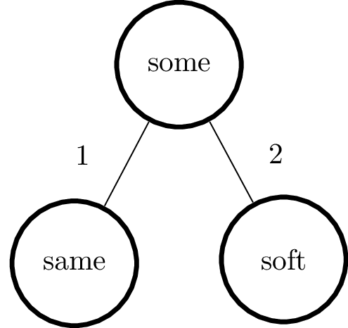
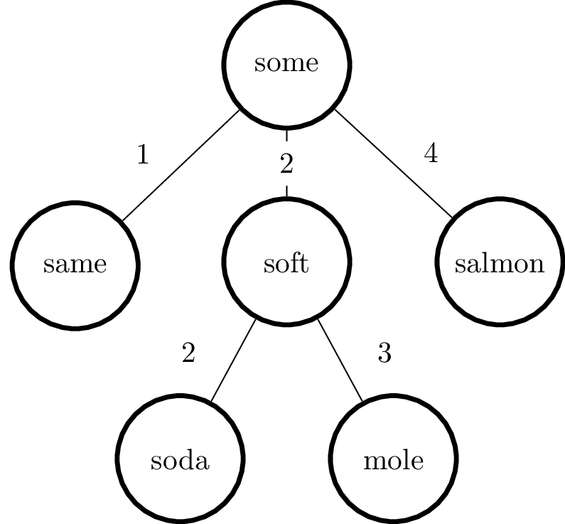
because the distance between “some” and “same” is $1$ and the distance between “some” and “soft” is $2$. Now, let’s add the next word, “mole”. Observe that the distance between “mole” and “some” is again $2$, so we add it to the tree as a child of “soft”, with an edge corresponding to their distance. After adding all the words we obtain the following tree:
Search
Remember that the original problem was to find all the words closest to a given query word. Call $N$ the maximum allowed distance (which we’ll call radius). The algorithm proceeds as follows:
- create a candidates list and add the root node to it
- take a candidate, compute its distance $D$ from the query key and compare it with the radius;
- selection criterion: add to the candidates list all the children of the current node that, from their parent, have a distance between $D - N$ and $D + N$ (inclusive).
Suppose we want to find all the words in our dictionary that are no more distant than $N = 2$ from the word “sort”. Our only candidate is the root node “some”. We start by computing
$$D = \mathop{\mathrm{Levenshtein}}(\text{‘sort’}, \text{‘some’}) = 2$$
Since the radius is $2,$ we add “some” to the list of results. Then we extend our candidates list with all the children that have a distance from the root node between $D - N = 0$ and $D + N = 4$. In this case, all the children satisfy this condition. Moving on, we compute
$$D = \mathop{\mathrm{Levenshtein}}(\text{‘sort’}, \text{‘same’}) = 3$$
Since $D > N$, this node is not a result and we move on to “soft”; now
$$D = \mathop{\mathrm{Levenshtein}}(\text{‘sort’}, \text{‘soft’}) = 1$$
Hence “soft” is an acceptable result. Regarding its children, we take those that have a distance between $D - N = -1$ and $D + N = 3$. Again, all of them, but only “soda” is a valid result. Finally, “salmon” is not acceptable. If we sort our results by distance we end up with the following:
[(1, 'soft'), (2, 'some'), (2, 'soda')]
Why does it work?
It’s interesting to understand why we are allowed to prune all the children that do not meet the criterion we gave above in point $3$. In the introduction we said that our distance function $d$ must satisfy a set of axioms in order for us to obtain the metric space structure. Those axioms are the following. For all elements $a,b,c$ it must hold:
- non-negativity: $d(a, b) \ge 0$;
- $d(a, b) = 0$ implies $a = b$ (and vice-versa);
- symmetry: $d(a, b) = d(b, a)$
- triangle inequality: $d(a, b) \le d(a, c) + d(c, b)$.
The first three are just a formalization of our intuitive notion of “distance”, while the last one derives from the relation between sides of a triangle in Euclidean geometry. This is often the most difficult property to demonstrate when we want to prove that a generic distance is actually a metric. As it turns out, the Levenshtein distance satisfies this property and therefore it’s a metric. This is why we can use it in the examples above.
Let’s call the query key $\bar x$. Suppose we are evaluating the child $B$ of an arbitrary node $A$ inside the tree, which we calculated to be at a distance $D = d(\bar x, A)$ from the query key. This situation is summarized in the following figure:
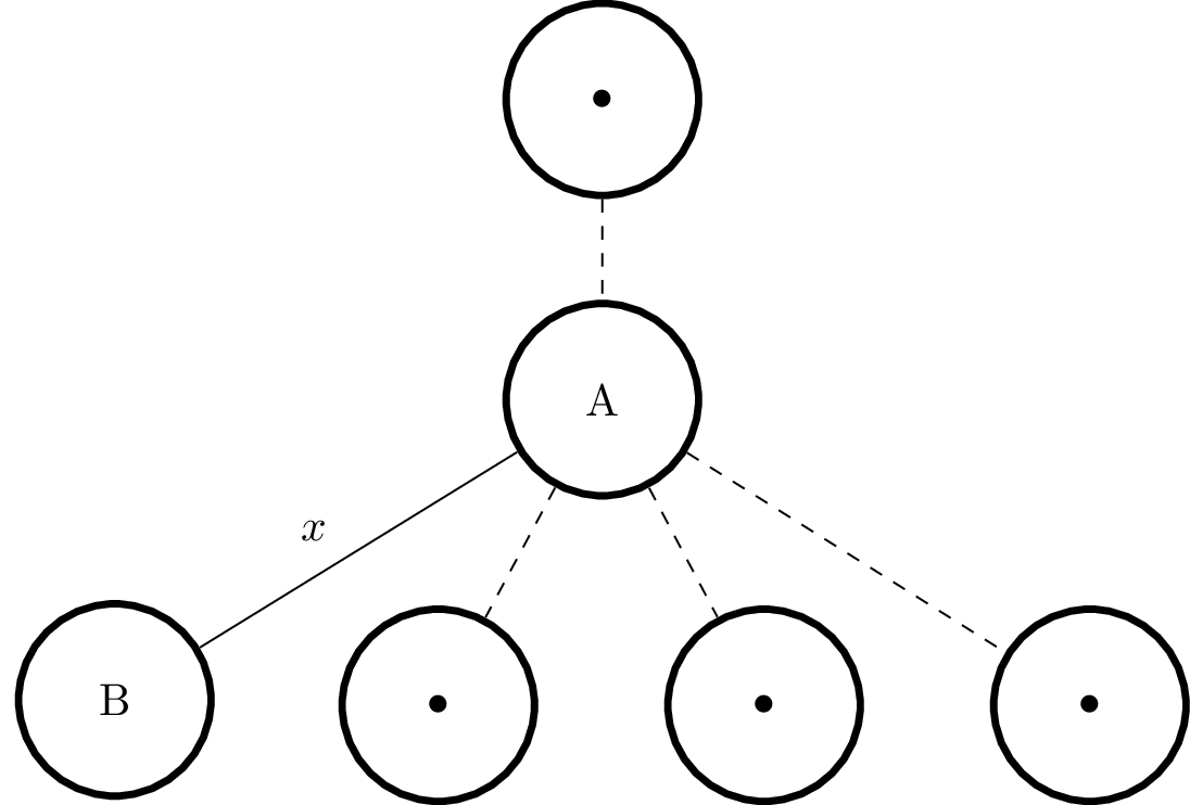
Since we assumed that $d$ is a metric, by the triangle inequality we have
$$d(A, B) \le d(A, \bar x) + d(\bar x, B)$$
from which
$$d(\bar x, B) \ge d(A, B) - d(A, \bar x) = x - D.$$
Using the triangle inequality again, this time with $d(A, \bar x)$ and $B$, we obtain
$$d(\bar x, B) \ge d(A, \bar x) - d(A, B) = D - x$$
Since we are only interested in nodes that are at a distance at most $N$ from the query key $\bar x$, we impose the constraint $d(\bar x, B) \le N$. This translates to
$$\begin{cases}x - D \le N\\ D - x \le N\end{cases}$$
which is equivalent to
$$D - N \le x \le D + N$$
We have proved that if $d$ is a metric, we can safely discard nodes that do not meet the above criteria. Finally, note that every child of $B$ will be at a distance of $x$ from $A$ (by construction of the BK-tree) and therefore we can safely prune the whole sub-tree if $B$ alone does not meet the criterion.
Implementation
This data structure is easy to implement in Python, if we use dictionaries to represent edges.
from collections import deque


class BKTree:
    def __init__(self, distance_func):
        self._tree = None
        self._distance_func = distance_func

    def add(self, node):
        if self._tree is None:
            self._tree = (node, {})
            return

        current, children = self._tree
        while True:
            dist = self._distance_func(node, current)
            target = children.get(dist)
            if target is None:
                children[dist] = (node, {})
                break
            current, children = target

    def search(self, node, radius):
        if self._tree is None:
            return []

        candidates = deque([self._tree])
        result = []
        while candidates:
            candidate, children = candidates.popleft()
            dist = self._distance_func(node, candidate)
            if dist <= radius:
                result.append((dist, candidate))

            low, high = dist - radius, dist + radius
            candidates.extend(c for d, c in children.items()
                              if low <= d <= high)
        return result
The implementation is pretty straightforward and adheres completely to the algorithm we explained above. A few comments:
- there’s no need to add a
rootargument to the__init__method, since any element can be a root node. In our case the first one added will become root; - why is
dequeeven needed? At first I used aset, only to see it fail because dictionaries aren’t hashable. We need another data structure that allows $O(1)$ popping and linear insertion. Built-indeque, being a doubly-linked list, is a natural fit.
Conclusion
The BK-tree is a relatively lesser-known data structure suitable for nearest neighbor search (NNS). It allows a considerable reduction of the search space, if the distance we are working with is a metric. In practice, the speed improvement we get from pruning sub-trees heavily depends on the search space and the radius we select. This is why some experimentation is usually needed for the problem at hand. One area in which BK-tree does well is spell-checking: as long as one keeps the radius to $1$ or $2$ the search space is often reduced to under $10%$ of the original.